PNGRB- Petroleum and Natural Gas Regulatory Board पेट्रोलियम एवं प्राकृतिक गैस विनियामक बोर्ड

 

Welcome to the world of MS-EXCEL

PNGRB  Outline of  Syllabus

40 Hrs Training = 20 classes [Each class is of  2 hours]

Popularly used  Shortcut keys in MS-Excel

1) Ctrl + Shift + N ==> to insert a new sheet to existing workbook

2) Alt =       ==> for Autosum

3) Alt+H+O+I   ==> it will automatically adjust the column width

4) Alt+H+O+A  ==> it will automatically adjust the Row width

5) Ctrl+T ==> create table

6) Ctrl + G ==> to open Go to Dialogue box

7) Ctrl + E  ==> flash fill [version dependency is there and is based on pattern used  ]

8) Ctrl + Q ==> Create chart

9) Ctrl + shift + Enter ==> for applying transpose [version dependency is there ]

10) F5 ==> to open Go to dialogue box

11) Shift + F2 ==> to insert a Comment into your sheet

12) Shift + F10 ==> to Open Right click dialogue box

13) Window +D  ==> Minimize all  opened windows at once

14) Ctrl + Page up / down ==> to switch across different worksheet of current workbook

15) Ctrl + Home  ==> to directly Go to cell A1 

16) Ctrl + 9 ==> Hide row

17) Shift +Ctrl +9 ==> Unhide row

18) Ctrl + 0 ==> Hide column

19) Shift +Ctrl +0 ==> Unhide Column

20) Shift + Ctrl+ plus sign ==> To insert blank row

20) Ctrl+ Minus sign ==> To delete row

21) Alt + Enter key ==> Add a line in a same cell 

22) Ctrl + W ==> To close the workbook

23) Ctrl + shift + Plus sign ==> To add a new column or even a new row also

24) Alt + F1 ==> use it to create a chart based on selected table

25) Ctrl + A > F5>special > Blank >Ctrl+ F9 to minimize workbook

26) Window + L ==> To Lock the system

 Microsoft Excel keyboard shortcuts

Before you proceed, note that the list is pretty long but it is by no means a complete list consisting of all the Excel shortcuts. However, I have picked out some of the most useful shortcuts, and we hope this would be worth your time.

1. Ctrl + N: To create a new workbook.

2. Ctrl + O: To open a saved workbook.

3. Ctrl + S: To save a workbook.

4. Ctrl + A: To select all the contents in a workbook.

5. Ctrl + B: To turn highlighted cells bold.

6. Ctrl + C: To copy cells that are highlighted.

7. Ctrl + D: To fill the selected cell with the content of the cell right above.

8. Ctrl + F: To search for anything in a workbook.

9. Ctrl + G: To jump to a certain area with a single command.

10. Ctrl + H: To find and replace cell contents.

11. Ctrl + I: To italicise cell contents.

12. Ctrl + K: To insert a hyperlink in a cell.

13. Ctrl + L: To open the create table dialog box.

14. Ctrl + P: To print a workbook.

15. Ctrl + R: To fill the selected cell with the content of the cell on the left.

16. Ctrl + U: To underline highlighted cells.

17. Ctrl + V: To paste anything that was copied.

18. Ctrl + W: To close your current workbook.

19. Ctrl + Z: To undo the last action.

20. Ctrl + 1: To format the cell contents.

21. Ctrl + 5: To put a strikethrough in a cell.

22. Ctrl + 8: To show the outline symbols.

23. Ctrl + 9: To hide a row.

24. Ctrl + 0: To hide a column.

25. Ctrl + Shift + :: To enter the current time in a cell.

26. Ctrl + ;: To enter the current date in a cell.

27. Ctrl + `: To change the view from displaying cell values to formulas.

28. Ctrl + ‘: To copy the formula from the cell above.

29. Ctrl + -: To delete columns or rows.

30. Ctrl + Shift + =: To insert columns and rows.

31. Ctrl + Shift + ~: To switch between displaying Excel formulas or their values in cell.

32. Ctrl + Shift + @: To apply time formatting.

33. Ctrl + Shift + !: To apply comma formatting.

34. Ctrl + Shift + $: To apply currency formatting.

35. Ctrl + Shift + #: To apply date formatting.

36. Ctrl + Shift + %: To apply percentage formatting.

37. Ctrl + Shift + &: To place borders around the selected cells.

38. Ctrl + Shift + _: To remove a border.

39. Ctrl + -: To delete a selected row or column.

40. Ctrl + Spacebar: To select an entire column.

41. Ctrl + Shift + Spacebar: To select an entire workbook.

42. Ctrl + Home: To redirect to cell A1.

43. Ctrl + Shift + Tab: To switch to the previous workbook.

44. Ctrl + Shift + F: To open the fonts menu under format cells.

45. Ctrl + Shift + O: To select the cells containing comments.

46. Ctrl + Drag: To drag and copy a cell or to a duplicate worksheet.

47. Ctrl + Shift + Drag: To drag and insert copy.

48. Ctrl + Up arrow: To go to the top most cell in a current column.

49. Ctrl + Down arrow: To jump to the last cell in a current column.

50. Ctrl + Right arrow: To go to the last cell in a selected row.

51. Ctrl + Left arrow: To jump back to the first cell in a selected row.

52. Ctrl + End: To go to the last cell in a workbook.

53. Alt + Page down: To move the screen towards the right.

54. Alt + Page Up: To move the screen towards the left.

55. Ctrl + F2: To open the print preview window.

56. Ctrl + F1: To expand or collapse the ribbon.

57. Alt: To open the access keys.

58. Tab: Move to the next cell.

59. Alt + F + T: To open the options.

60. Alt + Down arrow: To activate filters for cells.

61. F2: To edit a cell.

62. F3: To paste a cell name if the cells have been named.

63. Shift + F2: To add or edit a cell comment.

64. Alt + H + H: To select a fill colour.

65. Alt + H + B: To add a border.

66. Ctrl + 9: To hide the selected rows.

67. Ctrl + 0: To hide the selected columns.

68. Esc: To cancel an entry.

69. Enter: To complete the entry in a cell and move to the next one.

70. Shift + Right arrow: To extend the cell selection to the right.

71. Shift + Left arrow: To extend the cell selection to the left.

72. Shift + Space: To select the entire row.

73. Page up/ down: To move the screen up or down.

74. Alt + H: To go to the Home tab in Ribbon.

75. Alt + N: To go to the Insert tab in Ribbon.

76. Alt + P: To go to the Page Layout tab in Ribbon.

77. Alt + M: To go to the Formulas tab in Ribbon.

78. Alt + A: To go to the Data tab in Ribbon.

79. Alt + R: To go to the Review tab in Ribbon.

80. Alt + W: To go to the View tab in Ribbon.

81. Alt + Y: To open the Help tab in Ribbon.

82. Alt + Q: To quickly jump to search.

83. Alt + Enter: To start a new line in a current cell.

84. Shift + F3: To open the Insert function dialog box.

85. F9: To calculate workbooks.

86. Shift + F9: To calculate an active workbook.

87. Ctrl + Alt + F9: To force calculate all workbooks.

88. Ctrl + F3: To open the name manager.

89. Ctrl + Shift + F3: To create names from values in rows and columns.

90. Ctrl + Alt + +: To zoom in inside a workbook.

91. Ctrl + Alt +: To zoom out inside a workbook.

92. Alt + 1: To turn on Autosave.

93. Alt + 2: To save a workbook.

94. Alt + F + E: To export your workbook.

95. Alt + F + Z: To share your workbook.

96. Alt + F + C: To close and save your workbook.

97. Alt or F11: To turn key tips on or off.

98. Alt + Y + W: To know what's new in Microsoft Excel.

99. F1: To open Microsoft Excel help.

100. Ctrl + F4: To close Microsoft Excel.

Qs  Learn Excel Error Values

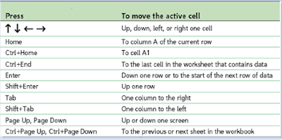
Qs  Practice all these Worksheet Navigation Keys.

 

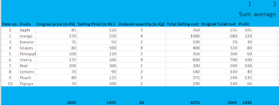
Create this file and save it as Fruits_Table 

Your Time Start Now - 10 Minutes

Download Fruits file from here

Frequently Used Excel Functions at Workplace

1)Sum( )

        (i) normal sum or Autosum or Alt =

        (ii) Sum with constant value

        (iii) Sum of random values

        (iv) Circular sum

2) Product( )                Example: =Product(5,4) 

3) Average( )               Example: = Average(a1:a10)           

4) Rept( )                    Example: =   Rept("PNGRB ",10)            

5) Power( )                 Example: =Power(2,3)

6) Concatenate( )       Example: =Concatenate("Petroleum ","Natural Gas")

7) Upper( )                 Example :  = Upper("amit")         Output : AMIT

8) Lower( )                Example :  =Lower("ANCHAL")        Output : anchal

9) Proper( )               Example :  =Proper("welcome to PNGRB") 

                                    Output : Welcome to Pngrb

                                       

10) Today( )   Try this one also  day(today) or  month(today) or year(today)  

11) Date( )             Example :  =date()

12) Year( )             Example :  =year(Today)

13) Month( )        Example :  =Month(Today)

14) Day( )            Example :  =Day(Today)

15) Now( )         It will display current date and time both

16) Hour( )    

17)Minute( )

18) Second( )

19) Len( )

20) Left( )

21) Right( )

22) Mid( )

23) Ltrim( )

24) Rtrim( )

25) Trim( )

26) Find( )

27) Replace( )

28) Search( )

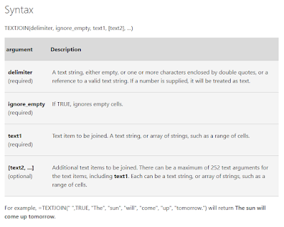
29) Textjoin( )                                             [see below chart first]

30) If ( )   

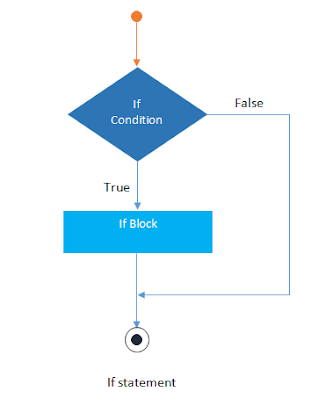
Understand the concept of If else Functions from this flow chart 

How does the IF() function in Excel work?

In Excel, the IF() function performs a logical test. It returns a value if the test evaluates to true and another value if the test result is false. It returns the value depending on whether the condition is valid for the entire selected range. 

 [Example : IF(B2=8,TRUE,FALSE) or IF(B2>=75,"You got Distinctions                            Congratulations!!…  ", "Your result is Average!!…")

              Example of Nested if means if inside another if conditions 

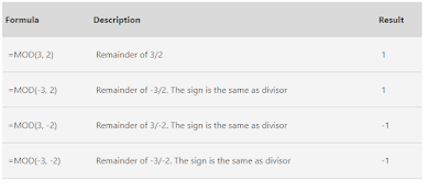
31) Mod( ) 

32) Fact( )

33) Count( ) 

34) Countblank ( )

35) CountA( )

36)Countif( )

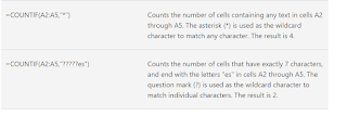
Use COUNTIF, one of the statistical functions, to count the number of cells that meet a criterion; for example, to count the number of times a particular city appears in a customer list.

In its simplest form, COUNTIF says:

=COUNTIF(Where do you want to look?, What do you want to look for?)

For example:

=COUNTIF(A2:A5,"London")

=COUNTIF(A2:A5,A4)

37) Subtotal( )

SUBTOTAL(function_num, ref1, [ref2],…)

Where:

Function_num - a number that specifies which function to use for the subtotal.

Ref1, Ref2, … - one or more cells or ranges to subtotal. 

The function_num argument can belong to one of the following sets:

1 - 11 ignore filtered-out cells, but include manually hidden rows.

101 - 111 ignore all hidden cells - filtered out and hidden manually.

38) Datedif( )       [see below chart first] 

Practice below examples

*******************************************************************

39 ) Vlookup( )

Download the data from here

Qs What is the use of VLOOKUP and how do we use it?

The function VLOOKUP in Excel is used to look up information in a table and extract the corresponding data.

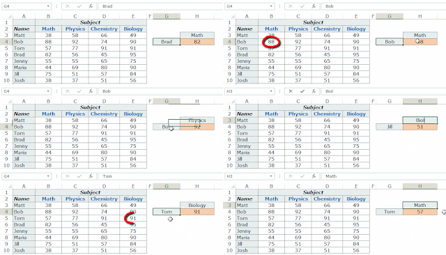
Here is the VLOOKUP formula that will return Brad’s Math score:

=VLOOKUP("Brad",$A$3:$E$10,2,0) 

or 

can use cell reference also instead of "Brad" 

=VLOOKUP(G3,$A$3:$E$10,2,0) 

To do this, you need to use the MATCH function as the column argument.

Here is the VLOOKUP formula that will do this:

=VLOOKUP(G4,$A$3:$E$10,MATCH(H3,$A$2:$E$2,0),0)

40) Hlookup ( )

41) Min( )

42) Max( )

 

43) Convert ( )

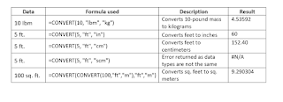
  LBM -  lean body mass                                                                                                   SCM -Standard Cubic Metre

44) Averageif ( )

45)Sumif ( )

46)Row()

47) Column()

48) Exact()           Example :' =exact("PNGRB","pngrb") ==> output : Faslse 

49) Info()             Example  : =INFO("RELEASE")    ==> Know the version of Excel

50) Char()

51) Code()

52) Cell()       Example " =cell( "Insert path of file here")

53) Create instant chart by simply pressing F11 key after selecting required datasheet

55)Even()    Example : Even(5)

56)ODD()     Example : ODD(18)

57) Press Ctrl + ' to see the used formulas 

58) T() it will check either the entered value is text or not if text then it will show you text else blank will appear.

How to use Arithmetic operators in Excel

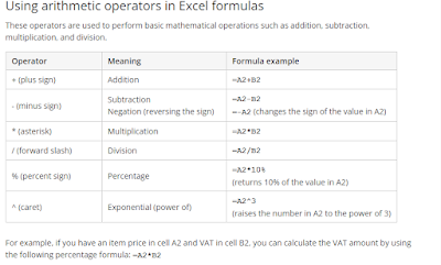
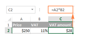
Let's understand how to apply comparison operators in Excel formulas

Create this table to implement PIVOT Table concept

How can you restrict someone from copying a cell from your worksheet?

1. First, choose the data you want to protect.

2. Hit Ctrl + Shift + F. The Format Cells tab appears. Go to the Protection tab. Check Locked and click OK.

3. Next, go to the Review tab and select Protect Sheet. Enter the password to protect the sheet. 

 

Qs What do you mean by Relative cell referencing and Absolute cell referencing in MS Excel?

Relative cell referencing

In Relative referencing, there is a change when copying a formula from one cell to another cell with respect to the destination. cells’ address 

This type of referencing is there by default. Relative cell referencing doesn’t require a dollar sign in the formula.

Absolute cell referencing 

Meanwhile, there is no change in Absolute cell referencing when a formula is copied, irrespective of the cell’s destination.

If you don’t want a change in the formula when it’s copied across cells, then absolute referencing requires you to add a dollar sign before and after the column and row address.

Formula	Function
The formula is like an equation in Excel, the user types in that. It can be any type of calculation depending on the user’s choice.	Whereas, a function in Excel is a predefined calculation which is in-built in Excel.
Manually typing out a formula every time you need to perform a calculation, consumes more time. Ex: = A1+A2+A3	However, performing calculations becomes more comfortable and faster while working with functions. Ex: = SUM(A1:A3)

Qs Mention the order of operations used in Excel while evaluating formulas.

The order of operations in Excel is referred to as PEDMAS. Shown below is the order of precedence while performing an Excel operation. 

1. Parentheses
2. Exponentiation
3. Division/Multiplication 
4. Addition
5. Subtraction

What is the shortcut to add a filter to a table?

The filter mechanism is used when you want to display only specific data from the entire dataset. By doing so, there is no change being made to the data. The shortcut to add a filter to a table is Ctrl+Shift+L

Qs How to find the formula cell ?

Ans: select the sheet first and then press CTRL +G > special > formulas> ok

Text concatenation operator

Text concatenation operator in Excel is the ampersand symbol (&). You can use it to join two or more text strings in a single string.

For example, if you have country codes in column A and telephone numbers in column B, you can use the following formula to get the telephone numbers combined with the country codes:

=A1&" "&B1

In the above formula, we concatenate a space " " in between to make the numbers better readable:

The same result can be achieved by using the CONCATENATE function.

What do you mean by "Excel formulas with nested functions" 

In Microsoft Excel formulas, nesting one function within another means using one function as an argument of another function. In modern versions of Excel 2016, 2013, 2010 and 2010, you can use up to 64 nested functions. In older versions of Excel 2003 and lower, only up to 7 levels of functions are allowed.

Here is a very simple example of a nested Excel formula that includes the SUM function to find the total, and ROUND function to round that number to the nearest integer (0 decimal places):

=ROUND(SUM(B2:B6),0)

******************************************************************************************************************************************

Why to go for charts ?

It is sometimes difficult to interpret the Excel data due to complexity and size of data. So, charts are a way to represent the data graphically and interpret the data easily. Charts are the visual representation of data.

Excel provides charts to take advantage of graphical representation. The data represented through charts is more understandable than the data stored in an Excel table. This makes the process of analyzing data fast. Excel users can fast analyze the data.

Excel charts 

                             Please download it as Excel file as amazon.xls

 Quiz Time

Qs How to calculate the Sum of negative and positive numbers in Excel?

Ans : use the formula Sumif for this. 

example : =SUMIF(D2:D11,">0",D2:D11) ==> for the sum of  positive numbers

                 =SUMIF(D2:D11,"<0",D2:D11)  ==> for the sum of negative numbers

Qs How to Merge Only Certain Parts of a Cell in Excel

Ans : =A1&" "&B1&" "&C1 Or can use Concatenate function OR use flash fills.

Format cells Shortcut keys

Qs What is circular sum in Excel

Ans . File > options > calculate options > manual or go to formulas tab and then calculate options > manual 

Qs  Use convert functions to change the data from one datatype to another datatype 

example hours to minutes and so on

QS What is the shortcut key for Autosum

Ans . Alt  =

QS use sequence function to automatically create a sequence up to 100

Ans =sequence(100)

try this one also =char(sequence(26,1,65) to generate a Sequence of  A to Z

Qs How to insert emojis in excel sheet ?

Ans : Simply press window icon along with dot from your keyboard black and white emojis will appear.

Please Note :) 

Press F9

The F9 key is a powerful tool that allows you to recalculate your worksheet. This shortcut is particularly useful when you have made changes to your data and need to update your calculations. Simply press F9, and Excel will recalculate all formulas in your worksheet.

Press Shift + F9

The Shift + F9 key calculates the Active worksheet. This shortcut is useful when you only need to update the data in the current worksheet.

Resources  : 

Case studies based on Excel usage

5 keyboard shortcuts to refresh your Excel worksheet (causal.app)

CONVERT function - Microsoft Support

https://trumpexcel.com/excel-vlookup-function/